
Red Hat OpenShift AI Intro/Pipelines
This article is a follow-up to the introductory post where we started with Workbenches in OpenShift AI (RHOAI). It assumes that you've already gone through those initial steps. At this point, you should have cloned the Git repository located at https://github.com/kcalliga/rhoai-demos?ref=myopenshiftblog.com and executed the notebook named 1_load_event.ipynb.
Now, we’re going to take that initial workflow and convert it into an RHOAI Pipeline. Before diving into the technical steps, let’s first highlight some of the key advantages that pipelines bring to the table:
🔁 Reusability
Pipelines make it easy to stitch together modular code snippets into a repeatable workflow. In this example, we’ll use the numbered Jupyter notebooks as individual steps in the pipeline. Instead of rewriting the same logic every time, you can reuse components like:
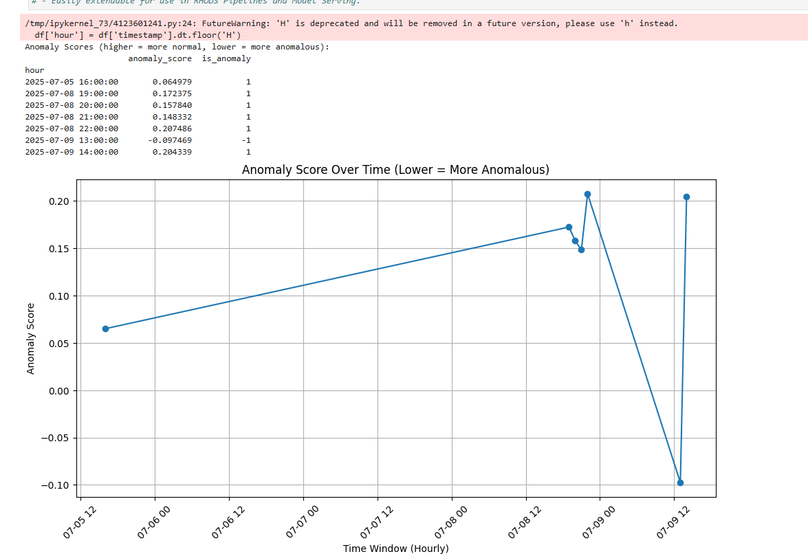
1_load_event.ipynbto load JSON-formatted event data from an OpenShift or Kubernetes cluster.2_rest_of_steps.ipynbto preprocess/clean data, apply TF-IDF vectorization, aggregate anomalies per hour, train Isolation Forest for anomaly detection (machine learning process), score and identify anomalies, and then display the results.
Each of the steps listed under the notebook called 2_rest_of_steps could be done separately but it is easier at this point to just show a two step pipeline since there is some manual steps required when doing this using Elyra (more on Elyra in a bit).
🧱 Modularity
Each notebook or step becomes a self-contained unit. This structure makes debugging and maintenance easier—if one step fails or needs improvement, you can isolate and iterate without affecting the rest of the pipeline.
🔗 Integration with Other RHOAI Features
Pipelines integrate smoothly with the broader OpenShift AI ecosystem. Once this pipeline is built, it can:
- Be reused by multiple team members working within the same RHOAI Project.
- Standardize workflows for model training, retraining, or serving.
- Act as part of a scheduled or event-driven retraining loop for model refreshes.
🤝 Collaboration and CI/CD
Using Git-based workflows, teams can collaborate on code updates, review changes, and trigger deployments based on version control events. New commits can automatically trigger pipeline runs—pulling in the latest production-ready logic for model training or inference.
Now, that we know the benefits to this, let's take the existing code and make a Pipeline out of this.
- From the main RHODS page, go to the project you would like to work on.
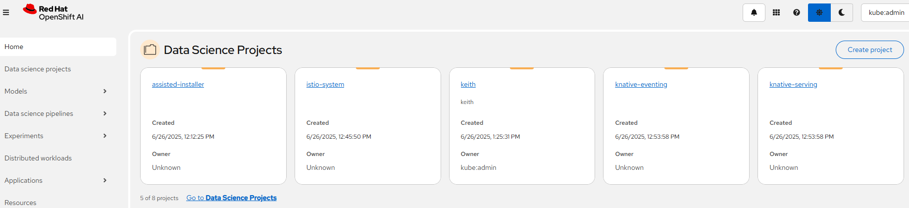
- On the left-hand side, click on Data science pipelines --> Pipelines
- If Pipelines server is not enabled, enable it.
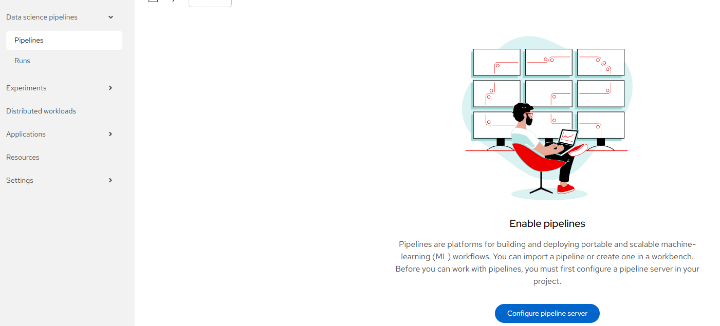
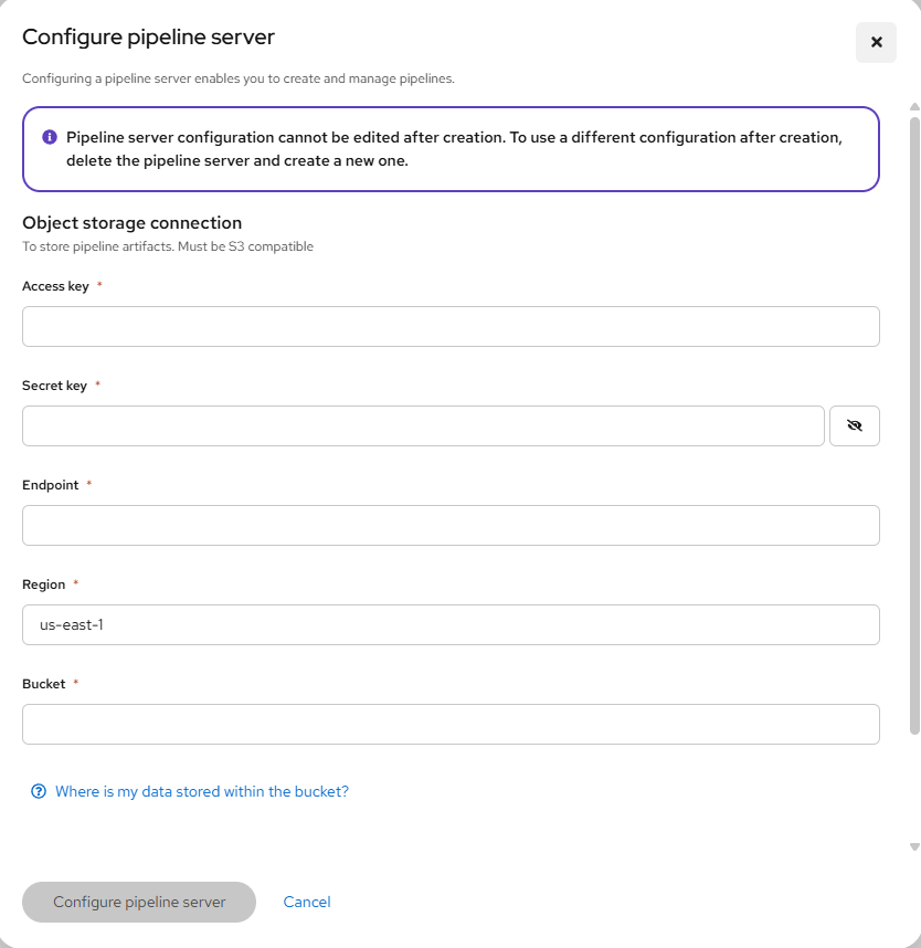
Click on "Configure pipeline server".
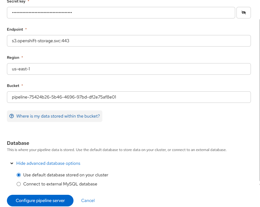
This will take you to a page that is asking for your S3 bucket information.
Go to step #4 if you don't have this. Otherwise, go to step #5
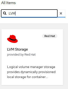
- Since this is a new pipeline server, let's create an S3 bucket in this project and reference this. The assumption here is that you have Openshift Data Foundation install available. If you need help enabling this functionality, see the following article:
- Fill-in the following values based on the S3 object claim (OBC) that you created.
Access-Key: From OBC
Secret-Key: From OBC
Endpoint: s3.openshift-storage.svc:443
Region: us-east-1
Bucket: From OBC
Leave the default database options as we will be creating a new database.
Click "Configure pipeline server".
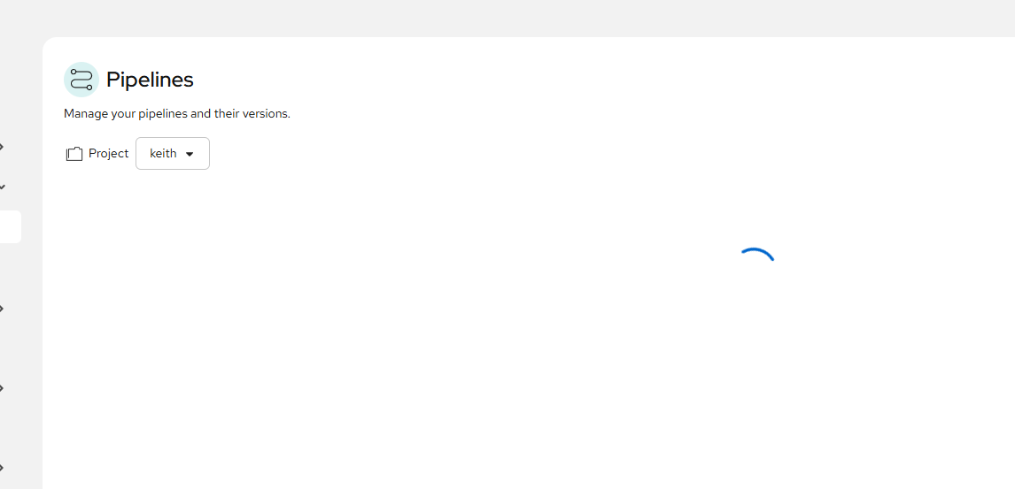
Wait for this to complete. This may take a few minutes. You will see something similar to the following:
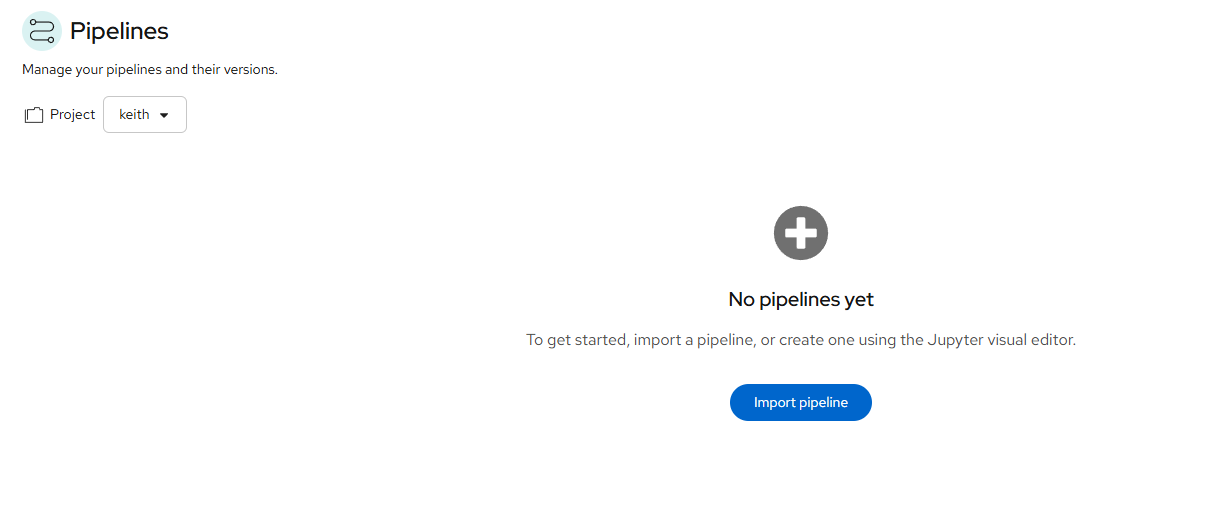
When finished, it will allow you to create a new Pipeline as shown below:
Before we input the pipeline, we need to convert these notebook as appropriate using Elyra.
- Open your workbench that you created previously. Mine was called test.
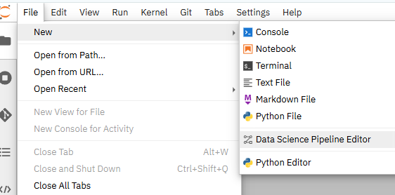
Once in that workbench, go to File --> New --> Data Science Pipeline Editor.
- You should now see a pipeline editor screen along with the rest of the notebooks you cloned from my repo.
- On the left-hand side, click on Gearbox/settings icon which is the "Runtimes" menu. On the screenshot below one run-time is already configured, but hit the "+" button to add a new one.
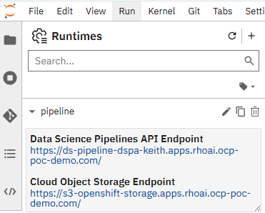
Set the following:
This is just an example:
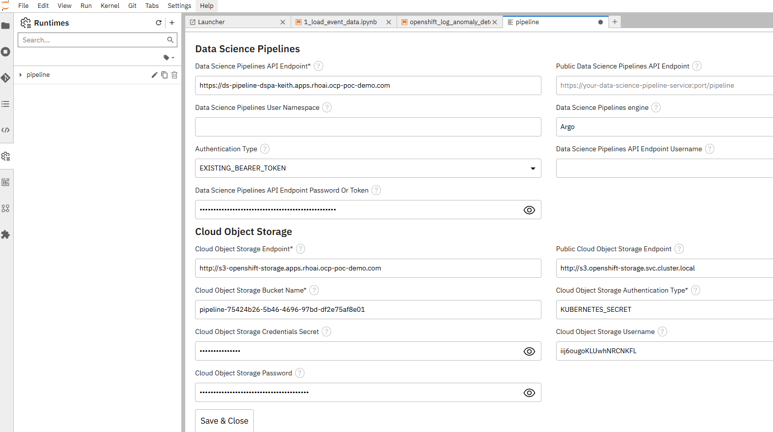
I realize that some of this information may appear redundant in this form, so I'm working on getting wording of these menus tweaked (and some other fixes).
For the S3 and Pipeline API endpoints, I used the route
For the pipeline-secret, I applied a YAML similar to the following:
apiVersion: v1
kind: Secret
metadata:
  name: pipeline-secret
  namespace: <your_namespace>
stringData:
  AWS_ACCESS_KEY_ID: <your access key id from OBC>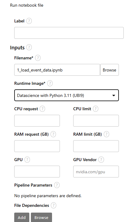
AWS_SECRET_ACCESS_KEY: <your secret access key from OBC>- Let's drag and drop the first notebook called 1_load_event_data.ipynb from the left-side of the screen to the middle frame (pipeline editor window).
Once you do this, you may see a message that a Runtime was not defined. Let's define this now.
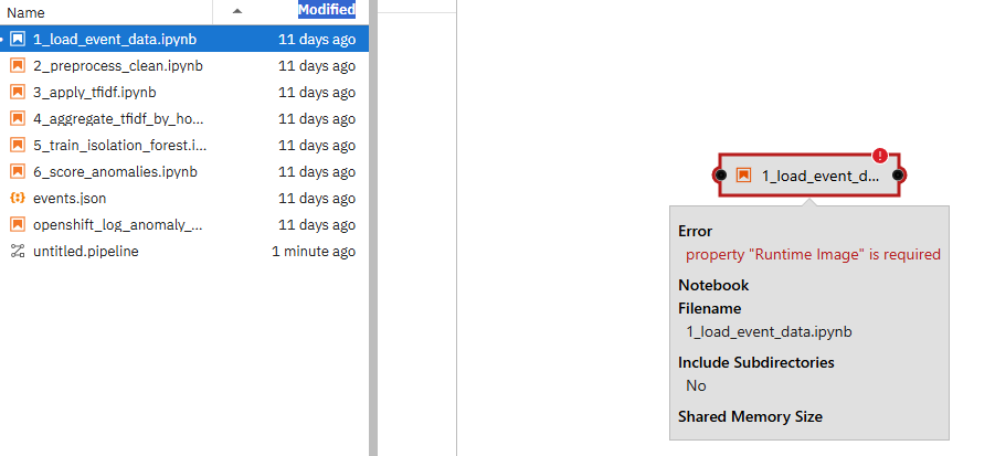
Right-click on the 1_load_event_data.ipynb box with red exclamation mark.
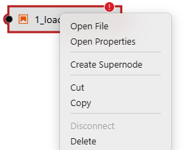
Go to "Open Properties"
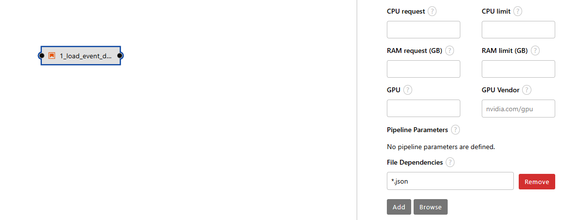
- Now, let's add some file dependencies and output file so step 1 (first node in pipeline) sends output to step 2 (second node of pipeline).
Under "Node Properties"
For file dependencies, use *.json to account for the events.json file.
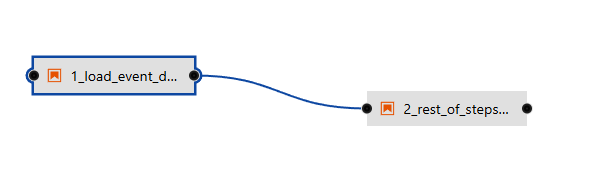
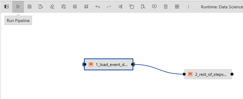
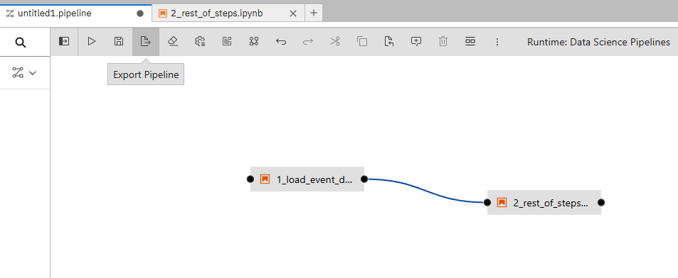
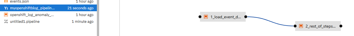
- Let's drag and drop the first notebook called 2_rest_of_steps.ipynb from the left-side of the screen to the middle frame (pipeline editor window).
Connect the output node for step1 to input of step2 as shown below.
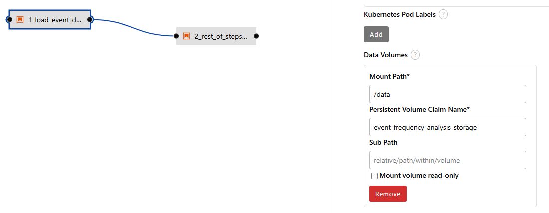
- Add the PVC mount associated with your project/workbench.
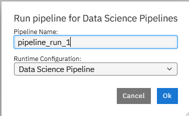
- Now, run the pipeline by hitting the play button.
- Once you run this a pop-up window should appear. Name it as you like and click "Ok".
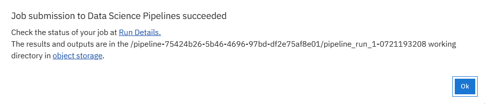
- You can now click on the "run details" or the object storage browser to see the outputs.
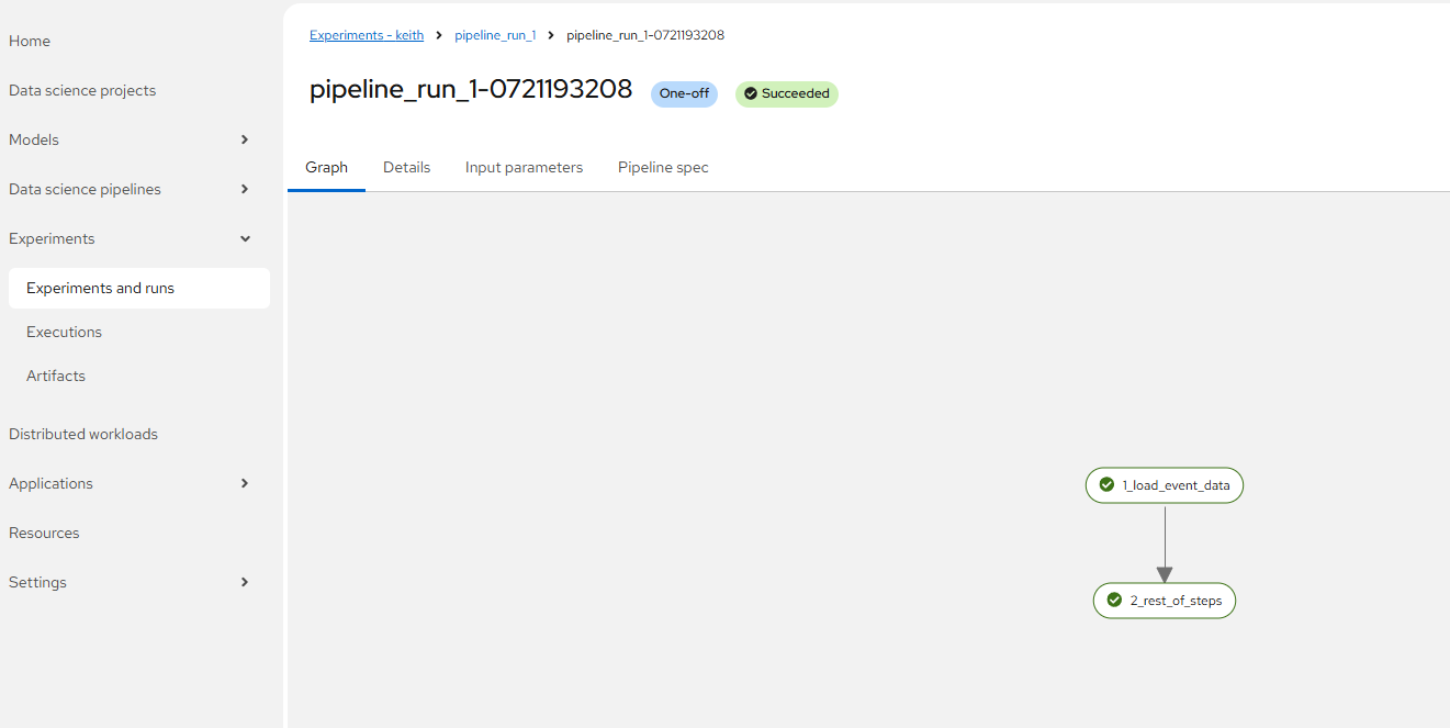
For run details, the screen will look as follows. This is assuming a good run.
For the object storage, you will see various outputs saved.
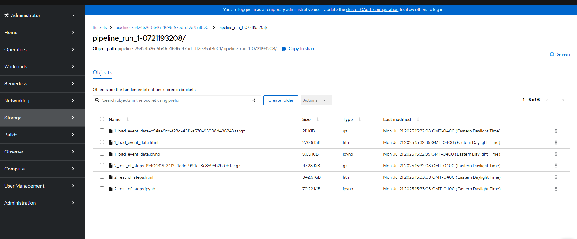
Your actual output file (csv) that gets saved from step #1 to step #2 is actually stored on the PVC so you will not see it here.
One thing you can see here is the html output from the second part of the Jupyter notebook run.
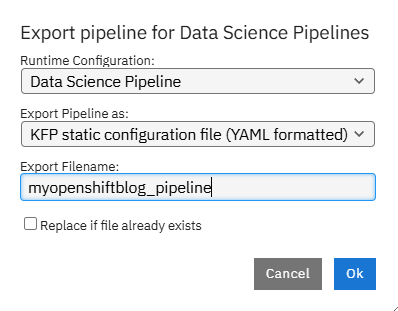
- The last thing I want to do is convert this to Kubeflow format (kfp) since this is more universally accepted.
Click on the "Export Pipeline" button.
You may be prompted to save.
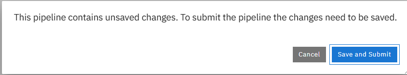
Click "Save and Submit"
Export as KFP YAML file and call the pipeline whatever you would like and this click "Ok".
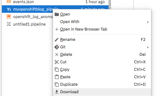
- You should now see the file on the left-hand menu.
Right-click and download.
- Now that this file is saved in KFP format, there is an easier way to create this whole pipeline.
- Back and the main Openshift AI dashboard, go to Data science pipelines menu and click Import pipeline.
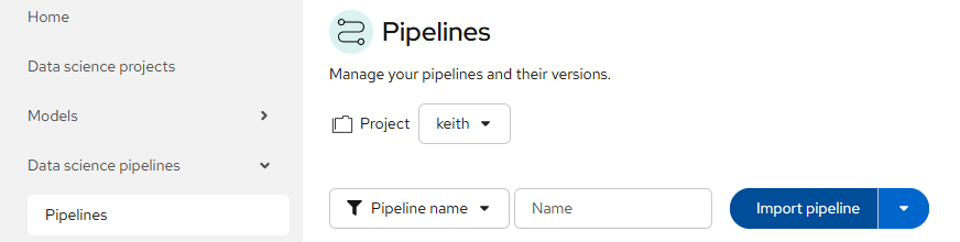
Provide and appropriate name/description and apply the myopenshiftblog_pipeline.yaml file you saved.
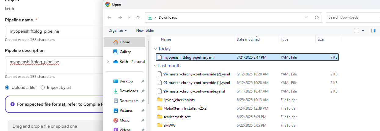
Click "Import Pipeline".
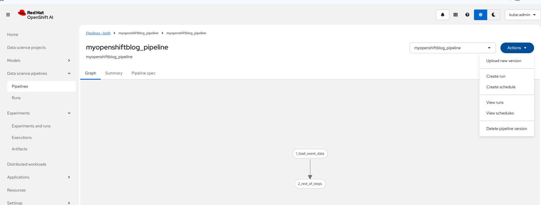
Now, the Kubeflow formatted pipeline has been imported into your RHOAI cluster.
If you want to quick-start this, you could follow the step #18 and import the YAML from my Github repo.
https://github.com/kcalliga/rhoai-demos/blob/main/myopenshiftblog_pipeline.yaml
The only requirement would be to clone my Git repo as shown in the previous workbench article.
Hope you enjoyed this. Next, we will get into model-serving.